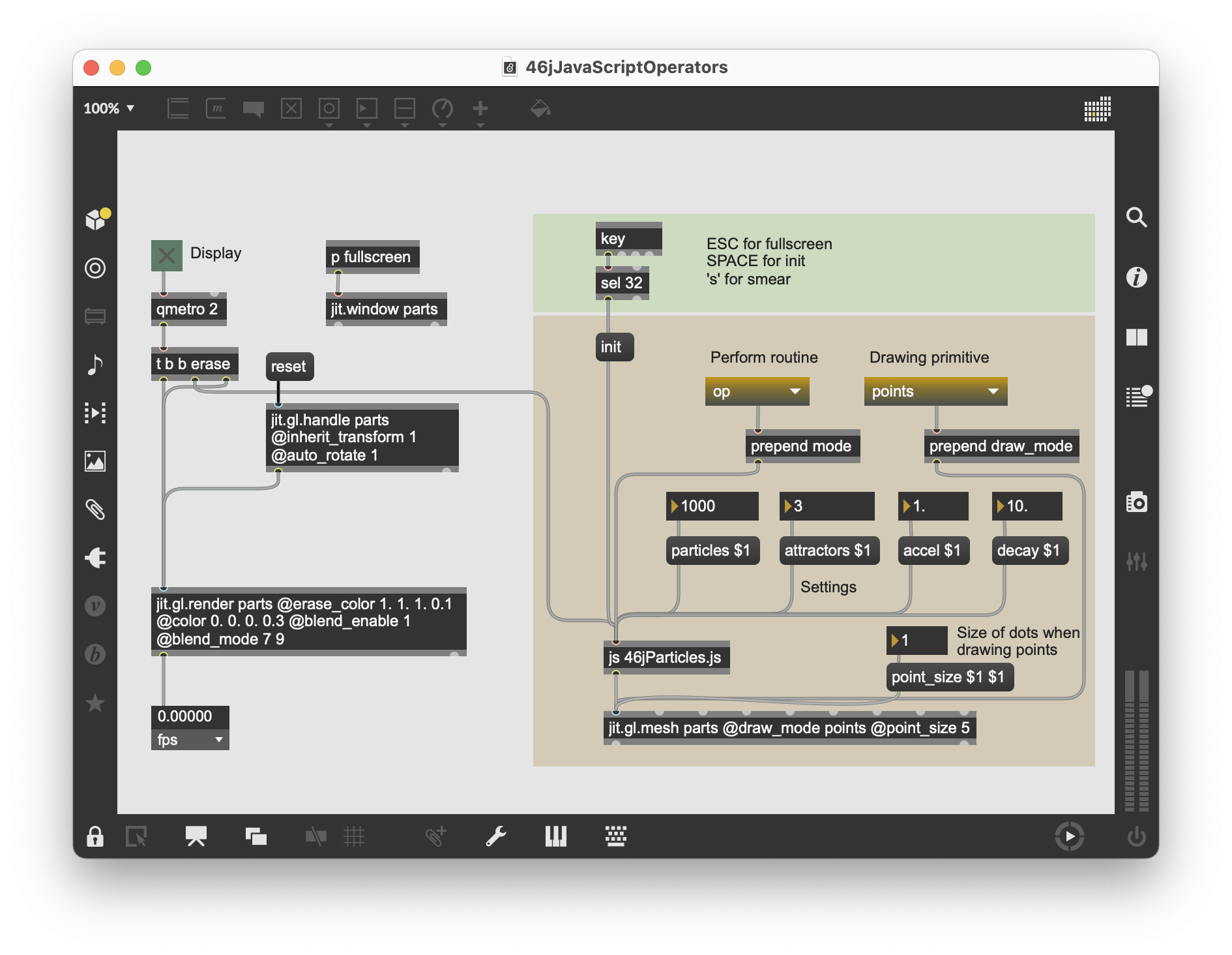
 Our patcher containing the JavaScript file.
As we saw in the last tutorial, we can use the Max
This tutorial assumes you've read through the previous Tutorial 45: Introduction to using Jitter within JavaScript. In addition, this tutorial works with Jitter OpenGL objects as well as
This tutorial patch uses a
Our patcher containing the JavaScript file.Our JavaScript code generates a set of points that represent a simple particle system. A particle system is essentially an algorithm that operates on a (often very large) number of spatial points called particles. These particles have rules that determine how they move over time in relation to each other or in relation to other actors within the space. At their basic level, particles contain only their spatial coordinates. Particle systems may also contain other information and can be used to simulate a wide variety of natural processes such as running water or smoke. Particle systems are widely used in computer simulations of our environment, and as such are a staple technology in many computer-generated imagery (CGI) applications.
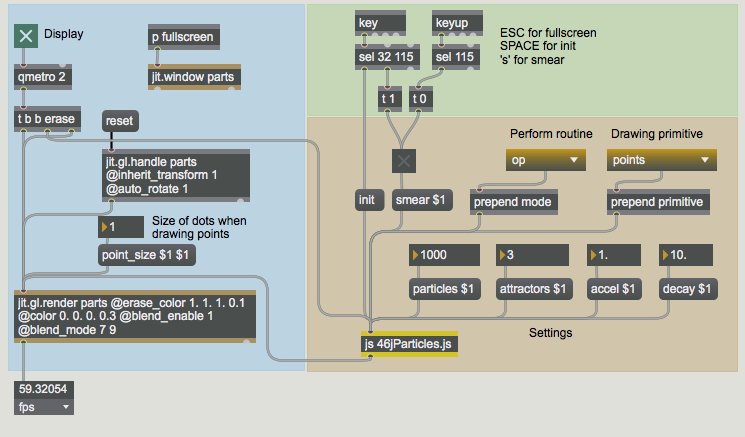
 A particle system generated as a Jitter matrix.
The particle system used in our JavaScript simulation works by generating two sets of random points representing the positions and velocities of the particles and a number of spatial positions in the 3D space that contain gravity. These gravity points, called attractors, act upon the particles in each frame to gradually pull particles towards them. As we can see in the
The
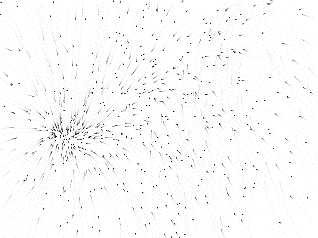
 A variety of behaviors from a simple set of rules.
A
Now that we've seen a good part of the functionality of the patch (we'll return to it later), let's look at the JavaScript code to see how the algorithm is constructed.
Our JavaScript code works by manipulating our particles and attractors as Jitter matrices. The particle system is updated by a generation every time our
After the initial comment block and inlet/outlet declarations, we can see a number of variables declared and initialized, including a few JitterObject and JitterMatrix objects. If we examine this code in detail, we can see the outline of how we'll perform our particle system.
var PARTICLE_COUNT = 1000; // initial number of particle vertices
var ATTRACTOR_COUNT = 3; // initial number of points of gravity
These two global variables (PARTICLE_COUNT and ATTRACTOR_COUNT) are used to decide how many particles and how many points of attraction we'd like to work with in our simulation. These will determine the
// create a [jit.noise] object for particle and velocity generation
var noisegen = new JitterObject("jit.noise");
noisegen.dim = PARTICLE_COUNT;
noisegen.planecount = 3;
noisegen.type = "float32";

// create a [jit.noise] object for attractor generation
var attgen = new JitterObject("jit.noise");
attgen.dim = ATTRACTOR_COUNT;
attgen.planecount = 3;
attgen.type = "float32";
Our particle systems are generated randomly by the init() function, which we will investigate presently. The
// create two [jit.expr] objects for the bang_expr() function
// first expression: sum all the planes in the input matrix
var myexpr = new JitterObject("jit.expr");
myexpr.expr = "in[0].p[0]+in[0].p[1]+in[0].p[2]";
// second expression: evaluate a+((b-c)*d/e)
var myexpr2 = new JitterObject("jit.expr");
myexpr2.expr = "in[0]+((in[1]-in[2])*in[3]/in[4])";
One of the ways we will update our particle system is to use two
// create the Jitter matrices we need to store our data
// matrix of x,y,z particle vertices
var particlemat = new JitterMatrix(3, "float32", PARTICLE_COUNT);
// matrix of x,y,z particle velocities
var velomat = new JitterMatrix(3, "float32", PARTICLE_COUNT);
// matrix of x,y,z points of attraction (gravity centers)
var attmat = new JitterMatrix(3, "float32", ATTRACTOR_COUNT);
// matrix for aggregate distances
var distmat = new JitterMatrix(3, "float32", PARTICLE_COUNT);
// temporary matrix for the bang_op() function
var tempmat = new JitterMatrix(3, "float32", PARTICLE_COUNT);
// temporary summing matrix for the bang_op() function
var summat = new JitterMatrix(1, "float32", PARTICLE_COUNT);
// another temporary summing matrix for the bang_op() function
var summat2 = new JitterMatrix(1, "float32", PARTICLE_COUNT);
// a scalar matrix to store the current gravity point
var scalarmat = new JitterMatrix(3, "float32", PARTICLE_COUNT);
// a scalar matrix to store acceleration (expr_op() function only)
var amat = new JitterMatrix(1, "float32", PARTICLE_COUNT);
Our algorithm calls for a number of JitterMatrix objects to store information about our particle system and to be used as intermediate storage during the processing of each generation of the system. The first three matrices (bound to the variables particlemat, velomat, and attmat) store the x,y,z positions of our particles, the x,y,z velocities of our particles, and the x,y,z positions of our attractors, respectively. The other six matrices are used in computing each generation of the system.
var a = 0.001; // acceleration factor
var d = 0.01; // decay factor
These two variables control two important aspects of the behavior of our particle system: the variable a controls how rapidly the particles accelerate toward an attractor, while the variable d controls how much the particles' current velocity decays with each generation. This second variable influences how easy it is for a particle to change direction and be drawn to other attractors.
var perform_mode="op"; // default perform functionThis variable defines which of the three techniques we'll use to process our particle system (the perform_mode).
The first step in creating a particle system is to generate an initial state for the particles and any factors that will act upon them (in our case, the attractor points). For example, were we to attempt to simulate a waterfall, we would start all our particles at the top of the space, with a fixed gravity field at the bottom of the space acting upon the particles with each generation. Our system is slightly less ambitious in terms of real-world accuracy—the particles and attractors will simply be in random positions throughout the 3D scene.
function loadbang() // execute this code when our Max patch opens
{
  init(); // initialize our matrices
  post("particles initialized.\n");
}

function init()
// initialization routine... call at load, as well as
// when we change the number of particles or attractors
{
  // generate a matrix of random particles spread between -1 and 1
  noisegen.matrixcalc(particlemat, particlemat);
  particlemat.op("*", 2.0);
  particlemat.op("-", 1.0);
  // generate a matrix of random velocities spread between -1 and 1
  noisegen.matrixcalc(velomat, velomat);
  velomat.op("*", 2.0);
  velomat.op("-", 1.0);
  // generate a matrix of random attractors spread between -1 and 1
  attgen.matrixcalc(attmat, attmat);
  attmat.op("*", 2.0);
  attmat.op("-", 1.0);
}
The loadbang() function in a
Our init() function runs when we open our patch as well as whenever we call it from our Max patcher (through the
Now that we have our initial state set up for our particle system, we need to look at how we process the particles with each generation. This is accomplished through one of three different methods in our JavaScript code determined by the perform_mode variable.
The
function bang() // perform one iteration of our particle system
{
  switch(perform_mode) { // choose from the following...
   case "op": // use Jitter matrix operators
      bang_op();
      break;
   case "expr": // use [jit.expr] for the bulk of the algorithm
      bang_expr();
      break;
   case "iter": // iterate cell-by-cell through the matrices
      bang_iter();
      break;
   default: // use bang_op() as our default
      bang_op();
      break;
  }
  // output our new matrix of particle vertices
  outlet(0, "jit_matrix", particlemat.name);
}
Our bang() function uses a JavaScript switch() statement to decide what function to call from within it to do the actual processing of our particle system. Depending on the perform_mode we choose in the Max patcher, we select from one of three different functions (bang_op(), bang_expr(), or bang_iter()). Assuming all goes well, we then output the message
In the grand tradition of Choose Your Own Adventure and Let's Make a Deal, we'll now investigate the three different perform routines represented by the different functions mentioned above.
Our bang_op() function updates our particle system by using, whenever possible, the op() method to the JitterMatrix object to mathematically alter the contents of matrices all at once. Whenever possible, we do this processing in place to limit the number of separate Jitter matrices we need to get through the algorithm. We perform the bulk of the processing multiple times within a for() loop, once for each attractor in our particle system. Once this loop completes, we get an updated version of the velocity matrix (velomat), which we then add to the particle matrix (particlemat) to define the new positions of the particles.
In a nutshell, we do the following:
function bang_op() // create our particle matrix using Matrix operators
{
  for(var i = 0; i < ATTRACTOR_COUNT; i++)
  // do one iteration per gravity point
  {
We perform the code until the closing brace (}) once for every attractor, setting the attractor we're currently working on to the variable i.
// create a scalar matrix out of the current attractor:
scalarmat.setall(attmat.getcell(i));
The getcell() method of a JitterMatrix object returns the values of the numbers in the cell specified as its argument. The setall() method sets all the cells of a matrix to a value (or array of values). These methods work the same as the corresponding messages to the
// subtract our particle positions from the current attractor
// and store in a temporary matrix (x,y,z):
tempmat.op("-", scalarmat, particlemat);
This code subtracts our particle positions (particlemat) from the position of the attractor we"re currently working with (scalarmat). The result is then stored in a temporary matrix with the same
// square to create a cartesian distance matrix (x*x, y*y, z*z):
distmat.op("*", tempmat, tempmat);
This code multiplies the tempmat matrix by itself, as a simple way of squaring it. The result is then stored in the distmat matrix.
// sum the planes of the distance matrix (x*x+y*y+z*z)
summat.planemap = 0;
summat.frommatrix(distmat);
summat2.planemap = 1;
summat2.frommatrix(distmat);
summat.op("+", summat, summat2);
summat2.planemap = 2;
summat2.frommatrix(distmat);
summat.op("+", summat, summat2);
In this block of code, we take the separate planes of the distmat matrix and add them together into a single-plane matrix called summat. In order to do this, we use the
// scale our distances by the acceleration value:
tempmat.op("*", a);
// divide our distances by the sum of the distances
// to derive gravity for this frame:
tempmat.op("/", summat);
// add to the current velocity bearings to get the
// amount of motion for this frame:
velomat.op("+", tempmat);
}
This is the last block of code in our per-attractor loop. We multiply the tempmat matrix (which contains the distances of our particles from the current attractor) by the value stored in the variable a, representing acceleration. We then divide that result by the summat matrix (the sum of the squared distances), and add those results to the current velocities of each particle as stored in the velomat matrix. The result of the addition is stored in velomat.
This entire process is repeated again for each attractor. As a result, the velomat matrix is added to each time based on how far our particles are from each attractor. By the time the loop finishes (when i reaches the last attractor index), velomat contains a matrix of velocities corresponding to the aggregate pull of all our attractors on all our particles.
   // offset our current positions by the amount of motion:
   particlemat.op("+", velomat);
   // reduce our velocities by the decay factor for the next frame:
   velomat.op("*", d);
}
Finally, we add these velocities to our matrix of particles (particlemat + velomat). Our particle matrix is now updated to a new set of particle positions. We then decay the velocity matrix by the amount stored in the variable d, so that the simulation retains a remnant of this generation"s velocity for the next generation of the particle system.
The use of a cascading series of op() methods to perform our algorithm on entire matrices gives us a big advantage in terms for speed, as Jitter can perform a simple mathematical operation on a large set of data very quickly. However, there are a few points (particularly in the generation of the summing matrix summat) where the code may have seemed more awkward than necessary. We can use
// create two [jit.expr] objects for the bang_expr() function

// first expression: sum all the planes in the input matrix
var myexpr = new JitterObject("jit.expr");
myexpr.expr = "in[0].p[0]+in[0].p[1]+in[0].p[2]";
// second expression: evaluate a+((b-c)*d/e)
var myexpr2 = new JitterObject("jit.expr");
myexpr2.expr = "in[0]+((in[1]-in[2])*in[3]/in[4])";
At the beginning of our JavaScript code we created two JitterObject objects (myexpr and myexpr2) that instantiated
A+((B-C)*D/E)
The basic outline of our bang_expr() function is equivalent to the bang_op() function, i.e. we iterate through a loop based on the number of attractors in our simulation, eventually ending up with an aggregate velocity matrix (velomat) that we than use to offset our particle matrix (particlemat). The key difference lies in where we insert the calls to
function bang_expr() // create our particle matrix using [jit.expr]
{
  // create a scalar matrix out of our acceleration value:
  amat.setall(a);
The above line fills every cell in the amat matrix with the value of the variable a (the acceleration factor). This allows us to use it as an operand in one of the
for(var i = 0; i < ATTRACTOR_COUNT; i++)
// do one iteration per gravity point
{
   // create a scalar matrix out of the current attractor:
   scalarmat.setall(attmat.getcell(i));
   // subtract our particle positions from the current attractor
   // and store in a temporary matrix (x,y,z):
   tempmat.op("-", scalarmat, particlemat);
   // square to create a cartesian distance matrix (x*x, y*y, z*z):
   distmat.op("*", tempmat, tempmat);
This is all the same as in bang_op(). We derive a squared distance matrix based on the difference between the current attractor and our particle positions.
// sum the planes of the distance matrix (x*x+y*y+z*z) :
// "in[0].p[0]+in[0].p[1]+in[0].p[2]" :
myexpr.matrixcalc(distmat, summat);
Instead of summing the distmat matrix plane-by-plane using op() and frommatrix() methods, we simply evaluate our first mathematical expression using distmat as a 3-plane input matrix and summat as a 1-plane output matrix.
// derive amount of motion for this frame :
// "in[0]+((in[1]-in[2])*in[3]/in[4])" :
myexpr2.matrixcalc([velomat,scalarmat,particlemat,amat,summat],velomat);
Similarly, at the end of our attractor loop we can derive the velocity matrix velomat in one compound expression based on the previous velocity matrix (velomat), the scalar matrix containing the current attractor point (scalarmat), the current particle positions (particlemat), the scalar matrix containing the acceleration (amat), and the matrix containing the distance sums (summat). This is much simpler (and a cleaner read) than using a whole sequence of op() functions working with intermediary matrices. Note that we use brackets ([ and ]) to establish an array of input matrices in the matrixcalc() method to the myexpr2 object.
   // offset our current positions by the amount of motion:
   particlemat.op("+", velomat);
   // reduce our velocities by the decay factor for the next frame:
   velomat.op("*", d);
}
This is the same as in bang_op(). We generate the new particle positions and decay the new velocities for use as initial velocities in the next generation of the system.
The bang_iter() function works in a different way from the other two perform routines we're using in our JavaScript code. Rather than working on the matrices as single entities, we work on everything on a cell-by-cell basis, iterating through not only the matrix of attractor positions (attmat), but also through the matrices of particles and velocities. We do this through a pair of nested for() loops, temporarily storing each cell value in different Array objects. We use the getcell() and setcell1d() methods to the JitterMatrix object to retrieve and store values from these Arrays.
function bang_iter() // create our particle matrix cell-by-cell
{
  var p_array = new Array(3); // array for a single particle
  var v_array = new Array(3); // array for a single velocity
  var a_array = new Array(3); // array for a single attractor

  for(var j = 0; j < PARTICLE_COUNT; j++)
  // do one iteration per particle
  {
   // fill an array with the current particle:
   p_array = particlemat.getcell(j);
   // fill an array with the current particle's velocity:
   v_array = velomat.getcell(j);

   for(var i = 0; i < ATTRACTOR_COUNT; i++)
   // do one iteration per gravity point
   {
      // fill an array with the current attractor:
      a_array = attmat.getcell(i);

      // find the distance from this particle to the
      // current attractor:
      var distsum = (a_array[0]-p_array[0])*(a_array[0]-p_array[0]);
      distsum+= (a_array[1]-p_array[1])*(a_array[1]-p_array[1]);
      distsum+= (a_array[2]-p_array[2])*(a_array[2]-p_array[2]);

      // derive the amount of motion for this frame:
      v_array[0]+= (a_array[0]-p_array[0])*a/distsum; // x
      v_array[1]+= (a_array[1]-p_array[1])*a/distsum; // y
      v_array[2]+= (a_array[2]-p_array[2])*a/distsum; // z
   }

   // offset our current positions by the amount of motion
   p_array[0]+=v_array[0]; // x
   p_array[1]+=v_array[1]; // y
   p_array[2]+=v_array[2]; // z

   // reduce our velocities by the decay factor for the next frame:
   v_array[0]*=d; // x
   v_array[1]*=d; // y
   v_array[2]*=d; // z

   // set the position for this particle in the Jitter matrix:
   particlemat.setcell1d(j, p_array[0],p_array[1],p_array[2]);
   // set the velocity for this particle in the Jitter matrix:
   velomat.setcell1d(j, v_array[0],v_array[1],v_array[2]);
  }
}
Note that by updating our particle system bit-by-bit (and using intermediary Array objects to store data for each cell) we're essentially replicating the same operation, as many times as there are particles in our system! While this may not be noticeably inefficient with a small number of particles, once you begin to work with thousands of points it will become noticeably slower.
The bulk of these functions simply change variables, sometimes scaling them first (e.g. accel() and decay() simply change the values of a and d, respectively). Similarly, the mode() function changes the value of the perform_mode variable to a string that we use to decide the perform routine:
function mode(v) // change perform mode
{
  perform_mode = v;
}
The particles() and attractors() functions, however, need to not only change the value of a variable (PARTICLE_COUNT and ATTRACTOR_COUNT, respectively), but they need to change the
function particles(v) // change the number of particles we're working with
{
  PARTICLE_COUNT = v;

  // resize matrices
  noisegen.dim = PARTICLE_COUNT;
  particlemat.dim = PARTICLE_COUNT;
  velomat.dim = PARTICLE_COUNT;
  distmat.dim = PARTICLE_COUNT;
  attmat.dim = PARTICLE_COUNT;
  tempmat.dim = PARTICLE_COUNT;
  summat.dim = PARTICLE_COUNT;
  summat2.dim = PARTICLE_COUNT;
  scalarmat.dim = PARTICLE_COUNT;
  amat.dim = PARTICLE_COUNT;

  init(); // re-initialize particle system
}

function attractors(v)
// change the number of gravity points we're working with
{
  ATTRACTOR_COUNT = v;

  // resize attractor matrix
  attgen.dim = ATTRACTOR_COUNT;

  init(); // re-initialize particle system
}Our particle system is visualized by sending the matrix of particle positions (referred to as particlemat in our JavaScript code) to the
For more information on the specifics of these drawing primitives and the OpenGL matrix format, consult Appendix B: The OpenGL Matrix Format or the OpenGL "Redbook".
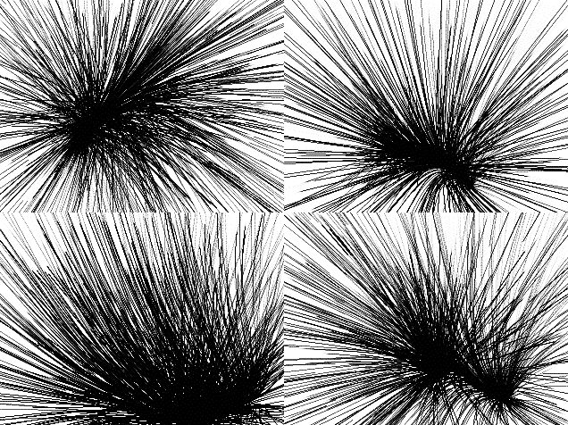
 Different ways of visualizing our particles using different drawing primitives.
 JavaScript can be a powerful language to use when designing algorithms that manipulate matrix data in Jitter. The ability to perform mathematical operations directly on matrices using a variety of techniques (op() methods,
In the next tutorial, we"ll look at ways to trigger callback functions in JavaScript based on the actions of JitterObject objects themselves.
// 46jParticles.js
//
// a 3-D particle generator with simple gravity simulation
// demonstrating different techniques for mathematical
// matrix manipulation using Jitter objects in [js].
//
// rld, 7.05
//

inlets = 1;
outlets = 1;

var PARTICLE_COUNT = 1000; // initial number of particle vertices
var ATTRACTOR_COUNT = 3; // initial number of points of gravity

// create a [jit.noise] object for particle and velocity generation
var noisegen = new JitterObject("jit.noise");
noisegen.dim = PARTICLE_COUNT;
noisegen.planecount = 3;
noisegen.type = "float32";

// create a [jit.noise] object for attractor generation
var attgen = new JitterObject("jit.noise");
attgen.dim = ATTRACTOR_COUNT;
attgen.planecount = 3;
attgen.type = "float32";

// create two [jit.expr] objects for the bang_expr() function

// first expression: sum all the planes in the input matrix
var myexpr = new JitterObject("jit.expr");
myexpr.expr = "in[0].p[0]+in[0].p[1]+in[0].p[2]";
// second expression: evaluate a+((b-c)*d/e)
var myexpr2 = new JitterObject("jit.expr");
myexpr2.expr = "in[0]+((in[1]-in[2])*in[3]/in[4])";

// create the Jitter matrices we need to store our data

// matrix of x,y,z particle vertices
var particlemat = new JitterMatrix(3, "float32", PARTICLE_COUNT);
// matrix of x,y,z particle velocities
var velomat = new JitterMatrix(3, "float32", PARTICLE_COUNT);
// matrix of x,y,z points of attraction (gravity centers)
var attmat = new JitterMatrix(3, "float32", ATTRACTOR_COUNT);
// matrix for aggregate distances
var distmat = new JitterMatrix(3, "float32", PARTICLE_COUNT);
// temporary matrix for the bang_op() function
var tempmat = new JitterMatrix(3, "float32", PARTICLE_COUNT);
// temporary summing matrix for the bang_op() function
var summat = new JitterMatrix(1, "float32", PARTICLE_COUNT);
// another temporary summing matrix for the bang_op() function
var summat2 = new JitterMatrix(1, "float32", PARTICLE_COUNT);
// a scalar matrix to store the current gravity point
var scalarmat = new JitterMatrix(3, "float32", PARTICLE_COUNT);
// a scalar matrix to store acceleration (expr_op() function only)
var amat = new JitterMatrix(1, "float32", PARTICLE_COUNT);

var a = 0.001; // acceleration factor
var d = 0.01; // decay factor

var perform_mode=""op";" // default perform function

function loadbang() // execute this code when our Max patch opens
{
  init(); // initialize our matrices
  post("particles initialized.\n");
}

function init()
// initialization routine... call at load, as well as
// when we change the number of particles or attractors
{
  // generate a matrix of random particles spread between -1 and 1
  noisegen.matrixcalc(particlemat, particlemat);
  particlemat.op("*", 2.0);
  particlemat.op("-", 1.0);
  // generate a matrix of random velocities spread between -1 and 1
  noisegen.matrixcalc(velomat, velomat);
  velomat.op("*", 2.0);
  velomat.op("-", 1.0);
  // generate a matrix of random attractors spread between -1 and 1
  attgen.matrixcalc(attmat, attmat);
  attmat.op("*", 2.0);
  attmat.op("-", 1.0);
}

function bang() // perform one iteration of our particle system
{
  switch(perform_mode) { // choose from the following...
   case "op": // use Jitter matrix operators
      bang_op();
      break;
   case "expr": // use [jit.expr] for the bulk of the algorithm
      bang_expr();
      break;
   case "iter": // iterate cell-by-cell through the matrices
      bang_iter();
      break;
   default: // use bang_op() as our default
      bang_op();
      break;
  }

  // output our new matrix of particle vertices
  outlet(0, "jit_matrix", particlemat.name);

}

function bang_op() // create our particle matrix using Matrix operators
{
  for(var i = 0; i < ATTRACTOR_COUNT; i++)
  // do one iteration per gravity point
  {
   // create a scalar matrix out of the current attractor:
   scalarmat.setall(attmat.getcell(i));

   // subtract our particle positions from the current attractor
   // and store in a temporary matrix (x,y,z):
   tempmat.op("-", scalarmat, particlemat);

   // square to create a cartesian distance matrix (x*x, y*y, z*z):
   distmat.op("*", tempmat, tempmat);

   // sum the planes of the distance matrix (x*x+y*y+z*z)
   summat.planemap = 0;
   summat.frommatrix(distmat);
   summat2.planemap = 1;
   summat.frommatrix(distmat);
   summat.op("+", summat, summat2);
   summat2.planemap = 2;
   summat2.frommatrix(distmat);
   summat.op("+", summat, summat2);

   // scale our distances by the acceleration value:
   tempmat.op("*", a);
   // divide our distances by the sum of the distances
   // to derive gravity for this frame:
   tempmat.op("/", summat);
   // add to the current velocity bearings to get the
   // amount of motion for this frame:
   velomat.op("+", tempmat);
  }

   // offset our current positions by the amount of motion:
   particlemat.op("+", velomat);
   // reduce our velocities by the decay factor for the next frame:
   velomat.op("*", d);
}

function bang_expr() // create our particle matrix using [jit.expr]
{
  // create a scalar matrix out of our acceleration value:
  amat.setall(a);

  for(var i = 0; i < ATTRACTOR_COUNT; i++)
  // do one iteration per gravity point
  {
   // create a scalar matrix out of the current attractor:
   scalarmat.setall(attmat.getcell(i));
   // subtract our particle positions from the current attractor
   // and store in a temporary matrix (x,y,z):
   tempmat.op("-", scalarmat, particlemat);
   // square to create a cartesian distance matrix (x*x, y*y, z*z):
   distmat.op("*", tempmat, tempmat);

// sum the planes of the distance matrix (x*x+y*y+z*z) :
// "in[0].p[0]+in[0].p[1]+in[0].p[2]" :
   myexpr.matrixcalc(distmat, summat);

   // derive amount of motion for this frame :
   // "in[0]+((in[1]-in[2])*in[3]/in[4])" :
   myexpr2.matrixcalc([velomat,scalarmat,particlemat,amat,summat],
   velomat);

   // offset our current positions by the amount of motion:
   particlemat.op("+", velomat);
   // reduce our velocities by the decay factor for the next frame:
   velomat.op("*", d);
}

function bang_iter() // create our particle matrix cell-by-cell
{
  var p_array = new Array(3); // array for a single particle
  var v_array = new Array(3); // array for a single velocity
  var a_array = new Array(3); // array for a single attractor

  for(var j = 0; j < PARTICLE_COUNT; j++)
  // do one iteration per particle
  {
   // fill an array with the current particle:
   p_array = particlemat.getcell(j);
   // fill an array with the current particle's velocity:
   v_array = velomat.getcell(j);

   for(var i = 0; i < ATTRACTOR_COUNT; i++)
   // do one iteration per gravity point
   {
      // fill an array with the current attractor:
      a_array = attmat.getcell(i);

      // find the distance from this particle to the
      // current attractor:
      var distsum = (a_array[0]-p_array[0])*(a_array[0]-p_array[0]);
      distsum+= (a_array[1]-p_array[1])*(a_array[1]-p_array[1]);
      distsum+= (a_array[2]-p_array[2])*(a_array[2]-p_array[2]);

      // derive the amount of motion for this frame:
      v_array[0]+= (a_array[0]-p_array[0])*a/distsum; // x
      v_array[1]+= (a_array[1]-p_array[1])*a/distsum; // y
      v_array[2]+= (a_array[2]-p_array[2])*a/distsum; // z
   }

   // offset our current positions by the amount of motion
   p_array[0]+=v_array[0]; // x
   p_array[1]+=v_array[1]; // y
   p_array[2]+=v_array[2]; // z

   // reduce our velocities by the decay factor for the next frame:
   v_array[0]*=d; // x
   v_array[1]*=d; // y
   v_array[2]*=d; // z

   // set the position for this particle in the Jitter matrix:
   particlemat.setcell1d(j, p_array[0],p_array[1],p_array[2]);
   // set the velocity for this particle in the Jitter matrix:
   velomat.setcell1d(j, v_array[0],v_array[1],v_array[2]);
  }
}


function particles(v) // change the number of particles we're working with
{
  PARTICLE_COUNT = v;

  // resize matrices
  noisegen.dim = PARTICLE_COUNT;
  particlemat.dim = PARTICLE_COUNT;
  velomat.dim = PARTICLE_COUNT;
  distmat.dim = PARTICLE_COUNT;
  attmat.dim = PARTICLE_COUNT;
  tempmat.dim = PARTICLE_COUNT;
  summat.dim = PARTICLE_COUNT;
  summat2.dim = PARTICLE_COUNT;
  scalarmat.dim = PARTICLE_COUNT;
  amat.dim = PARTICLE_COUNT;

  init(); // re-initialize particle system
}

function attractors(v)
// change the number of gravity points we're working with
{
  ATTRACTOR_COUNT = v;

  // resize attractor matrix
  attgen.dim = ATTRACTOR_COUNT;

  init(); // re-initialize particle system
}

function accel(v) // set acceleration
{
  a = v*0.001;
}

function decay(v) // set decay
{
  d = v*0.001;
}

function mode(v) // change perform mode
{
  perform_mode = v;
}

function bang() // perform one iteration of our particle system
{
  switch(perform_mode) { // choose from the following...
   case "op": // use Jitter matrix operators
      bang_op();
      break;
   case "expr": // use [jit.expr] for the bulk of the algorithm
      bang_expr();
      break;
   case "iter": // iterate cell-by-cell through the matrices
      bang_iter();
      break;
   default: // use bang_op() as our default
      bang_op();
      break;
  }

  // output our new matrix of particle vertices
  outlet(0, "jit_matrix", particlemat.name);

}

function bang_op() // create our particle matrix using Matrix operators
{
  for(var i = 0; i < ATTRACTOR_COUNT; i++) // do one iteration per gravity point
  {
   scalarmat.setall(attmat.getcell(i)); // create a scalar matrix out of the current attractor

   tempmat.op("-", scalarmat, particlemat); // subtract our particle positions from the current attractor and store in a temporary matrix (x,y,z)

   distmat.op("*", tempmat, tempmat); // square to create our cartesian distance matrix (x*x, y*y, z*z)

   // sum the planes of the distance matrix (x*x+y*y+z*z)
   summat.planemap = 0;
   summat.frommatrix(distmat);
   summat2.planemap = 1;
   summat.frommatrix(distmat);
   summat.op("+", summat, summat2);
   summat2.planemap = 2;
   summat2.frommatrix(distmat);
   summat.op("+", summat, summat2);

   tempmat.op("*", a); // scale our distances by the acceleration value
   tempmat.op("/", summat); // divide our distances by the sum of the distances to derive gravity for this frame
   velomat.op("+", tempmat); // add to the current velocity bearings to get the amount of motion for this frame
  }

   particlemat.op("+", velomat); // offset our current positions by the amount of motion
   velomat.op("*", d); // reduce our velocities by the decay factor for the next frame
}

function bang_expr() // create our particle matrix using [jit.expr]
{
  amat.setall(a); // create a scalar matrix out of our acceleration value

  for(var i = 0; i < ATTRACTOR_COUNT; i++) // do one iteration per gravity point
  {
   scalarmat.setall(attmat.getcell(i)); // create a scalar matrix out of the current attractor

   tempmat.op("-", scalarmat, particlemat); // subtract our particle positions from the current attractor and store in a temporary matrix (x,y,z)

   distmat.op("*", tempmat, tempmat); // square to create our cartesian distance matrix (x*x, y*y, z*z)

   myexpr.matrixcalc(distmat, summat); // sum the planes of the distance matrix (x*x+y*y+z*z) : "in[0].p[0]+in[0].p[1]+in[0].p[2]"

   myexpr2.matrixcalc([velomat,scalarmat,particlemat,amat,summat], velomat); // derive amount of motion for this frame : "in[0]+((in[1]-in[2])*in[3]/in[4])"
  }

   particlemat.op("+", velomat); // offset our current positions by the amount of motion
   velomat.op("*", d); // reduce our velocities by the decay factor for the next frame
}

function bang_iter() // create our particle matrix cell-by-cell
{
  var p_array = new Array(3); // create an array for a single particle (x,y,z)
  var v_array = new Array(3); // create an array for a single velocity (x,y,z)
  var a_array = new Array(3); // create an array for a single attractor (x,y,z)


  for(var j = 0; j < PARTICLE_COUNT; j++) // do one iteration per particle
  {
   p_array = particlemat.getcell(j); // fill an array with the current particle
   v_array = velomat.getcell(j); // fill an array with the current particle's velocity

   for(var i = 0; i < ATTRACTOR_COUNT; i++) // do one iteration per gravity point
   {
      a_array = attmat.getcell(i); // fill an array with the current attractor

      // find the distance from this particle to the current attractor
      var distsum = (a_array[0]-p_array[0])*(a_array[0]-p_array[0]);
      distsum+= (a_array[1]-p_array[1])*(a_array[1]-p_array[1]);
      distsum+= (a_array[2]-p_array[2])*(a_array[2]-p_array[2]);

      v_array[0]+= (a_array[0]-p_array[0])*a/distsum; // derive the amount of motion for this frame (x)
      v_array[1]+= (a_array[1]-p_array[1])*a/distsum; // derive the amount of motion for this frame (y)
      v_array[2]+= (a_array[2]-p_array[2])*a/distsum; // derive the amount of motion for this frame (z)
   }

   p_array[0]+=v_array[0]; // offset our current positions by the amount of motion (x)
   p_array[1]+=v_array[1]; // offset our current positions by the amount of motion (y)
   p_array[2]+=v_array[2]; // offset our current positions by the amount of motion (z)

   v_array[0]*=d; // reduce our velocities by the decay factor for the next frame (x)
   v_array[1]*=d; // reduce our velocities by the decay factor for the next frame (y)
   v_array[2]*=d; // reduce our velocities by the decay factor for the next frame (z)

   particlemat.setcell1d(j, p_array[0],p_array[1],p_array[2]); // set the position for this particle in the Jitter matrix
   velomat.setcell1d(j, v_array[0],v_array[1],v_array[2]); // set the velocity for this particle in the Jitter matrix
  }
}

function particles(v) // change the number of particles we're working with
{
  PARTICLE_COUNT = v;

  // resize matrices
  noisegen.dim = PARTICLE_COUNT;
  particlemat.dim = PARTICLE_COUNT;
  velomat.dim = PARTICLE_COUNT;
  distmat.dim = PARTICLE_COUNT;
  attmat.dim = PARTICLE_COUNT;
  tempmat.dim = PARTICLE_COUNT;
  summat.dim = PARTICLE_COUNT;
  summat2.dim = PARTICLE_COUNT;
  scalarmat.dim = PARTICLE_COUNT;
  amat.dim = PARTICLE_COUNT;

  init(); // re-initialize particle system
}

function attractors(v) // change the number of gravity points we're working with
{
  ATTRACTOR_COUNT = v;

  // resize attractor matrix
  attgen.dim = ATTRACTOR_COUNT;

  init(); // re-initialize particle system
}

function accel(v) // set acceleration
{
  a = v*0.001;
}

function decay(v) // set decay
{
  d = v*0.001;
}

function mode(v) // change perform mode
{
  perform_mode = v;
}