MSP Tutorials
Synthesis Tutorial 5: Waveshaping
In this tutorial, we'll look at a latent (but very useful)
attribute of samples, which is that they can be used as lookup
tables to transform the shape of other waveforms. This process
is called waveshaping, and is used in synthesis to generate
complex spectra from a sinusoidal input. It's also the basic signal
processing technique behind many types of amplitude-dependent distortion,
and can be used to model the non-linearities of different kinds of
amplifier.
Using a stored wavetable as a transfer function
Take a look at the tutorial patcher. The basic sound-generating
circuit in the upper-left of the patcher should look familiar, with
one new object (lookup~) inserted into the chain. We have
a cycle~ object going through an amplifier (*~) to
the ezdac~.
Turn on the ezdac~ object and adjust the number box
labeled amplitude. You should hear a sine wave at 220 Hz.
The new object in this signal chain at first seems to be doing
nothing, and in terms of what we hear, it isn't... yet.
The lookup~ object interprets a piece of sample memory
stored in a buffer~ object as a transfer function,
with the beginning of the sample used representing input values
of -1 and the end of the sample used representing values
of 1. Incoming values are scaled across this X axis,
and the resulting audio comes from the corresponding values along
the Y axis.
In our patch, the buffer~ named waveform is serving as
a lookup table (or transfer function) for the incoming sine
wave. When the cycle~ object generates a -1, for
example, whatever sample value is at the beginning of
the buffer~ comes out of the lookup~ object. When
our cycle~ hits 1, the lookup~ object reads
from the end of the buffer~ to find its outgoing sample.
Double-click the buffer~ object at the bottom of the tutorial
patcher. Notice that the waveform loaded in is a simple ramp. Because
our waveshape (the sample in the buffer~ is a linear ramp with
the beginning of the sample at -1 and the end at 1,
our cycle~ object sounds unchanged.
The lookup~ object takes three possible arguments: the first
is the name of the buffer~ to use as its waveshape; the second
and third are the start and end points (in samples to use
within the buffer~ as the boundaries of the transfer function.
Because we want our buffer~ to be exactly 512 samples
long in our patcher, we created it with the argument of 10.66667
milliseconds. How did we get this number. At the right of the patcher,
you can see the sampstoms~ object, which allows us to convert
from samples to milliseconds.
The waveform~ object
Look at the graphical object at the top of the tutorial patcher.
Notice that it contains the same shape that is loaded into our buffer~.
The waveform~ object allows us to view, select regions of, and
directly modify the contents of a buffer~ with a drawing tool.
Using your mouse, doodle in the waveform~ object's display.
Notice how different shapes affect the output sound. Try drawing
smooth curves, then jagged ones, then ones with lots of plateaus
(straight horizontal lines). Notice that even slight variations
in the shape have tremendous impact on the spectrum generated by
the lookup~ object.
The waveform~ object is operating in draw mode, where
you can literally modify a sample loaded into a buffer~ with
your mouse. Other modes allow you to select regions, the boundaries
of which can be used as Max messages for other objects.
Setting sample values with Max messages: peek~
Click on the button labeled A in the tutorial patcher.
Our waveshape (and our sound) should return to normal.
The way we got the default waveshape in our tutorial patcher is through the logic controlled by the uzi below the button labeled A. The uzi object, you may recall, generates a lot of data instantly depending on its argument. The right outlet of the object generates a numeric ramp from 1 to its argument. We've subtracted 1 from that value to generate a stream of Max numbers from 0 to 511 when you click the button. These numbers are then sent to the middle and left inlets of a peek~ object. The middle inlet receives a number that has been scaled into the range of -1 to 1 (via the scale object), then the left inlet receives the number unchanged. The peek~ object allows us to manually set the sample values within a buffer~ via Max messages. The left inlet (which is "hot", and actually performs the operation) sets which sample we're changing to the most recent value received by the middle inlet. In section A, the uzi object generates a stream of numbers that fill our entire buffer~ with an ascending ramp, e.g.
Sample Value
0 -1.
1 -0.996086
2 -0.992172
3 -0.988258
4 -0.984344
5 -0.980431
...
508 0.988258
509 0.992172
510 0.996086
511 1.
For the math geeks in the room
Click on the other button objects in the patcher
(labeled B, C, and D). Notice how the
waveshape in the buffer~ changes, and note how it affects
the sound. Each waveshape seems to multiply the frequency
of the sound generated by the cycle~ object. The logic
at B makes our 220 Hz wave sound at 440,
C at 660, and D at 880.
The equations that the expr objects are doing in these parts
of the patch generate special types of transfer functions
called Chebyshev polynomials. These functions are interesting
in that they have the ability to transform sinusoidal input to
different harmonic multiples. The four Chebyshev polynomials in our
tutorial are:
y = x (uzi object A, leaves the input unchanged)
y = 2*x^2-1 (uzi object B, doubles the frequency)
y = 4*x^3-3*x (uzi object C, triples the frequency)
y = 8*x^4-8*x^3+1 (uzi object D, quadruples the frequency)
In practice, what they do looks like this:
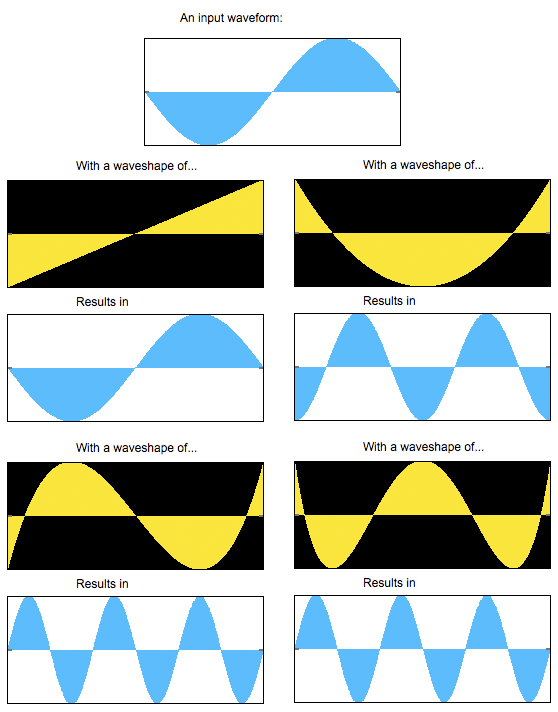 Our four Chebyshev polynomials and their effect on a cosine input
Click on the read messages in patcher area E. These will
load 512-sample audio files into our waveshape buffer~. Notice
their effect on the sound:
Our four Chebyshev polynomials and their effect on a cosine input
Click on the read messages in patcher area E. These will
load 512-sample audio files into our waveshape buffer~. Notice
their effect on the sound:
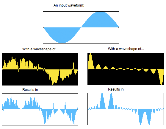 Waveshaping through gtr512.aiff and blp512.aiff, respectively.
Now that you know a bit more about the expected behavior of the
waveshaping distortion, return to drawing in the waveform~ object
to see what kind of results you can achieve.
Waveshaping through gtr512.aiff and blp512.aiff, respectively.
Now that you know a bit more about the expected behavior of the
waveshaping distortion, return to drawing in the waveform~ object
to see what kind of results you can achieve.
Summary
The lookup~ object allows you to use a buffer~ as a
transfer function to perform a process called waveshaping
on an input sound. Different shapes cause different distortions
of the spectra and can create very complex timbres. The waveform~
object allows you to directly view and modify the contents of an
MSP buffer~ using your mouse, and the peek~ object
allows you to set sample values programmatically with Max messages.
Some transfer functions (such as Chebyshev polynomials) have special
properties when used as a waveshaping function on a sinusoidal input.
Transfer function lookup table
buffer~ viewer and editor
Read and write sample values
Convert time from samples to milliseconds