Colorspaces
Jitter Java
Jitter Tutorials
Tutorial 50: Procedural Texturing & Modeling
In this Tutorial we will be examining different operations that can be used to construct a procedural model of a texture or some form of geometric data.
Procedural techniques are a powerful way of defining some aspect of a computer-generated model through algorithms and/or mathematical functions. In contrast to using pre-existing data such as a static images or photographs, procedural models can generate visual complexity of arbitrary resolution and infinite variation. In conjunction with parametric controls, such models can be used to build a flexible interface for controlling complex behaviors and capturing a special effect.
Jitter provides a comprehensive set of basis functions and generators that are exposed through the jit.bfg object. Each function performs a point-wise operation in n-dimensional space whose evaluation is independent of neighboring results. This means that these operations can be performed on any number of dimensions, across any coordinate, without any need of referencing existing calculations. In addition, since they all share a common interface, these objects can be combined together and evaluated in a function graph by cross-referencing several jit.bfg objects.
There are several categories of functions, each of which are characterized by a different intended use. These categories include fractal, noise, filter, transfer, and distance operations. Functions contained in these folders can be passed by name to jit.bfg either fully qualified (category.classname) or relaxed (classname).
Before looking at these categories in detail, we'll first explore the general interface of jit.bfg and show how to create different types of procedural functions and fill a jit.matrix with our results.
jit.bfg
Once the patch loads, take a look at the different objects being used. Notice that we have a metro object attached to the jit.bfg object. Once activated, a bang message will notify jit.bfg to evaluate and output a Jitter matrix just like most other Jitter objects. In this example, jit.bfg has been set up to generate a single plane matrix of type float32 and size 128x128.
Click on the toggle box connected to the metro object to begin sending bang messages to jit.bfg.
Notice that the jit.pwindow object remains solid black in color! Since jit.bfg has not been told what basis function evaluate, jit.bfg is not outputting a matrix and jit.pwindow remains unchanged.
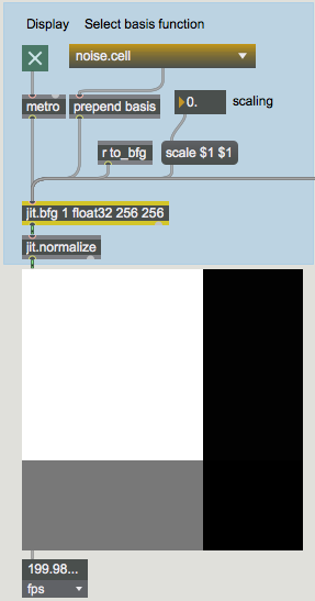
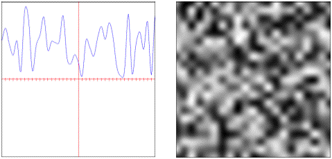
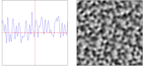
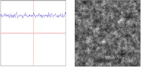
Select the noise.cell basis function from the list in the umenu object.
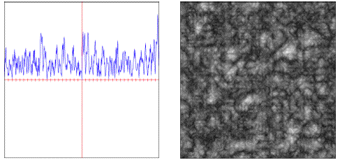
 An evaluated basis function.
Now that jit.bfg has been given a function to evaluate, we can see the results of its calculation in jit.pwindow. Internally, jit.bfg is generating a series of Cartesian coordinates that it passes to the indicated basis function during its evaluation.
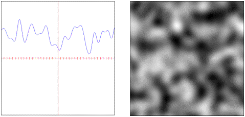
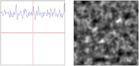
If we wanted to, we could adjust these coordinates and have jit.bfg perform the evaluation over a different domain.
Change the value of the number box connected to the scale message box.
Notice that the results of jit.bfg change as we adjust the domain.
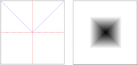
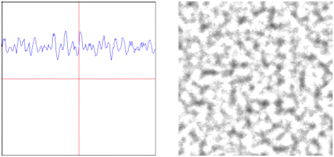
Select the distance.euclidean basis function from the list in the umenu object.
Again change the value of the number box connected to the scale message box.
Notice that positive values in the scale number box have little effect on the results being shown in jit.pwindow, whereas negative values flip the image components from white to black. What is going on? Distance should always be positive and increase outward from the origin, right?
jit.normalize
The output of jit.bfg goes into a jit.normalize object connected to the jit.pwindow. This object will examine an incoming matrix and scale the minimum and maximum values into a normalized range of 0-1.
When we changed the scale values being sent to jit.bfg for evaluating the distance.euclidean function from positive to negative, the highest and lowest values that were being outputted from jit.bfg switched as we crossed over the origin. Since jit.normalize always scales the input matrix maximum to 1 and the minimum to 0, our colors flipped.
Since the output range of jit.bfg may yield extremely large results, especially when evaluating unbounded functions such as fractals, we need to normalize our output in order to map the results for display.
Basis Categories
Now that we are familiar with the basic interface for setting up jit.bfg and specifying a basis function to evaluate, let's examine the contents of each function category.
Distance Functions
The functions in the distance category each define a unique metric for determining the positional difference from a given point to the global origin.
Descriptions of each of these functions are provided in the following list.
chebychev: Absolute maximum difference between two points.
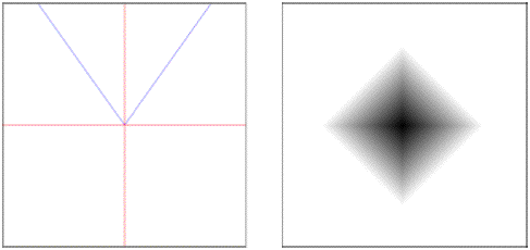
 euclidean: True straight line distance in Euclidean space.
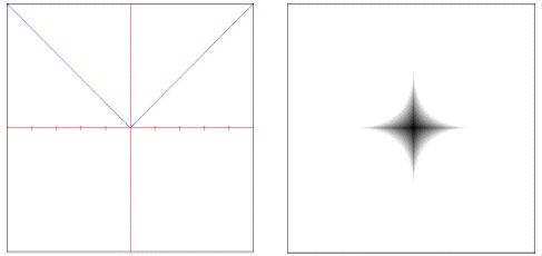
 euclidean.squared: Squared Euclidean distance.
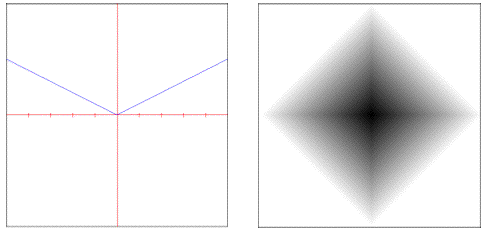
 manhattan: Rectilinear distance measured along axes at right angles.
 manhattan.radial: Manhattan distance with radius fall-off control.
 minkovsky: Exponentially controlled distance.
The noise.voronoi object requires one of these distance objects to be specified as part of its evaluation.
Filter Functions
The filter category contains signal processing filters which can be used to perform image sampling and reconstruction or to create pre-computed kernels for a general convolution.
Descriptions of each of these functions are provided in the following list.
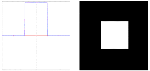
box: Sums all samples in the filter area with equal weight.
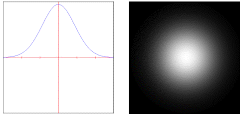
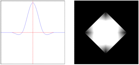
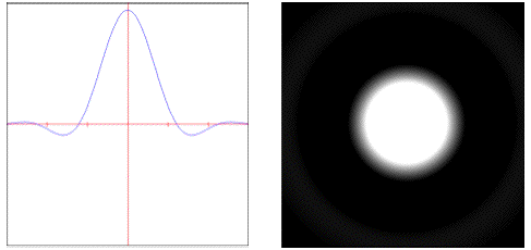
 gaussian: Weights samples in the filter area using a bell curve.
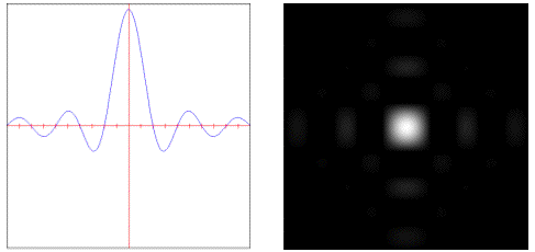
 lanczossinc: Weights samples using a steep windowed sinc curve.
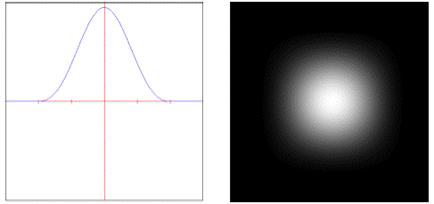 mitchell: Weights samples using a controllable cubic polynomial.
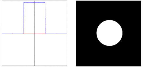
 disk: Sums all samples inside the filter's radius with equal weight.
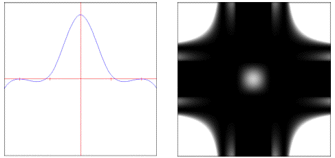
 sinc: Weights samples using an un-windowed sinc curve.
 catmullrom: Weights samples using a Catmull-Rom cubic polynomial.
 bessel: Weights samples with a linear phase response.
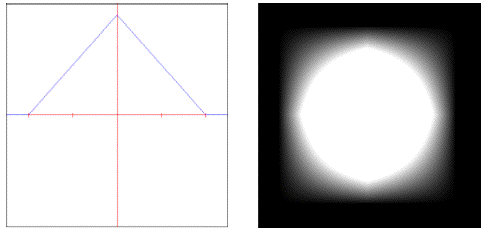
 triangle: Weights samples in the filter area using a pyramid.
These objects are used as parameters to both the noise.value.convolution and the noise.sparse.convolution objects, which expect to be given a filter object as part of their evaluation.
Transfer Functions
Functions that map input to a different output are contained in the transfer category. Most of these functions operate only on a single dimension within the unit interval 0-1.
A brief description of these functions is contained in the list below.
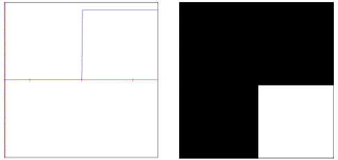
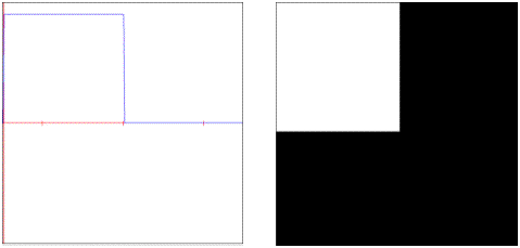
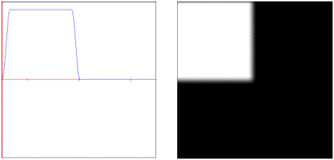
step: Always 1 if given value is less than threshold.
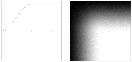
 smoothstep: Step function with cubic smoothing at boundaries.
 bias: Polynomial similar to gamma but remapped to unit interval.
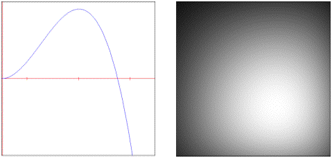
 cubic: Generic 3rd order polynomial with controllable coefficients.
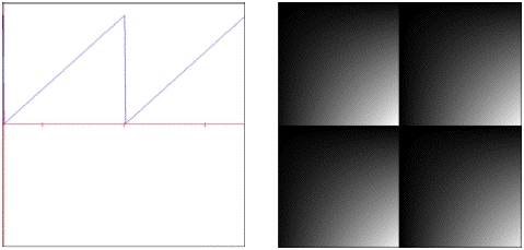
 saw: Periodic triangle pulse train.
 quintic: Generic 5th order polynomial with controllable coefficients.
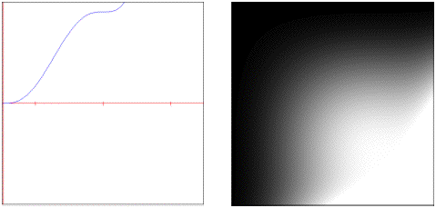 gain: S-Shaped polynomial evaluated inside unit interval. Note: the default settings will result in a linear curve instead of the descriptive S-curve shape.
 pulse: Periodic step function.
 smoothpulse: Periodic step function with cubic smoothing at boundaries.
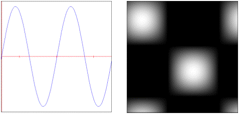
 sine: Periodic sinusoidal curve.
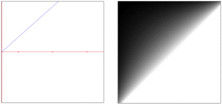
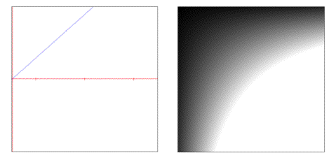
 linear: Linear function across unit interval.
solarize: Scales given value if threshold is exceeded.
linear: Linear function across unit interval.
solarize: Scales given value if threshold is exceeded.
These transfer functions can be used inside of several of the noise objects to change their smoothing function and/or alter their output.
Noise Functions
Deterministic stochastic patterns (aka pseudo-random coherent noise functions) are the cornerstone of nearly every procedural model. They allow a controllable amount of complexity to be created by adding visual detail.
A brief description of these functions is contained in the list below.
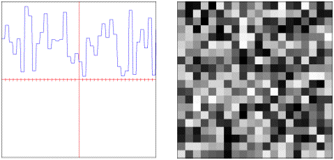
cellnoise: Coherent blocky noise.
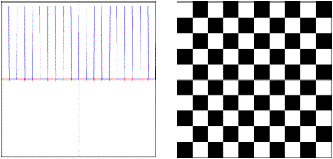
 checker: Periodic checker squares.
 value.cubicspline: Polynomial smoothed pseudo-random values.
 value.convolution: Convolution filtered pseudo-random values.
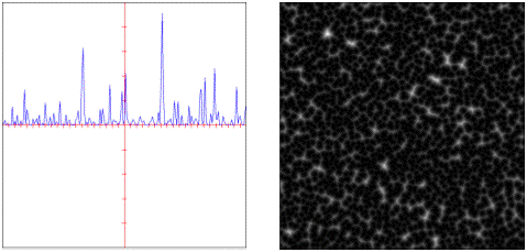
 sparse.convolution: Convolution filtered pseudo-random feature points.
 gradient: Directionally weighted polynomially interpolated values.
 simplex: Simplex weighted pseudo-random values.
 voronoi: Distance weighted pseudo-random feature points.
 distorted: Domain distorted combinational noise.
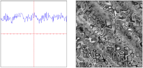
All of these functions are generators with the exception of the noise.distorted object, which is a binary operator and uses two existing functions for its evaluation.
Fractal Functions
Fractals provide a specialized form of generation by combining multiple scales or octaves of another basis function. This process forms the characteristic self-similarity exhibited by all fractals.
A brief description of these functions is contained in the list below.
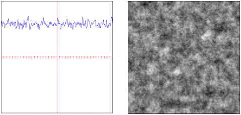
mono: Additive fractal with global simularity across scales.
 multi: Multiplicative fractal with varying simularity across scales.
 multi.hybrid: A hybrid additive and multiplicative fractal.
 multi.hetero: Heterogenous multiplicative fractal.
 multi.ridged: Multiplicative fractal with sharp ridges.
 turbulence: Additive mono-fractal with sharp ridges.
Other Attributes & Messages
Select the noise.checker basis function from the umenu object.
Notice that in addition to the scale message that we used previously, we can also transform the evaluation coordinates through rotation, translation (via offset) and by adjusting their origin.
Change the 1st and 2nd number boxes connected to origin to change the x and y origin.
Change the 1st and 2nd number boxes connected to offset to change the x and y offset position.
Change the 1st number box connected to rotation to change our rotation angle about the x axis.
Notice the effect of the transform. Also notice the drop in performance when a rotation is performed – we will always get better frame rates if the rotation attribute is left at 0 for each matrix dimension.
Technical Detail: In addition to the internal coordinate generation already described, jit.bfg also accepts an input matrix of coordinates to evaluate (XYZ map to planes 0-2, and the input matrix must be the same dim as the jit.bfg output matrix).
Change the 1st number box connected to rotation to 0 to disable rotation.
Click the toggle box connected to autocenter to enable automatic centering.
If the autocenter attribute is set to 1, the current matrix dim sizes will be used to place the origin in the center of the output matrix, overriding any values already set for the origin.
Click the toggle box connected to autocenter again to disable automatic centering.
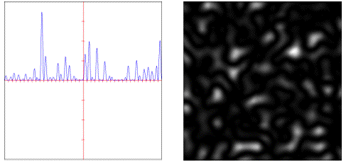
Select the noise.gradient basis function from the umenu object.
Click the dim 128 128 1 message box.
As mentioned previously, all of the basis functions that Jitter provides can be evaluated over any number of dimensions. This message has changed our output matrix to be a 3D matrix, and has correspondingly set the evaluation to be performed in 3-dimensional space. Since our display is still a 2D screen, we only need to evaluate a single slice in 3D, and thus our 3rd dim is set to 1.
Change the 3rd number box connected to offset to change the z evaluation position.
Notice how our results change. We are now traversing along the z-axis as if we were moving forward/backwards through a volume aligned with the screen.
Select float64 from the umenu connected to the precision message.
The precision message can be used to change the jit.bfg object’s internal evaluation precision. This may be desirable if we need more or less accurate results without changing the output matrix type.
Change the 3rd number box connected to offset to change the z evaluation position.
Notice how the higher precision affects the frame rate reported by the jit.fpsgui object. We should be careful to only use float64 precision when needed.
Select float32 from the umenu connected to the precision message.
Change the planecount for jit.bfg from 1 to 3 to enable RGB output.
In addition to n-dimensional evaluation, jit.bfg can generate up to 32 planes per dimension. Each plane is offset by a pseudo-random fractional amount controlled by the align attribute.
Change the number box connected to align for jit.bfg.
Notice how the planes separate and become more visible as the align amount gets larger.
To see more specific examples for different combinations of basis functions, open the help patch for the jit.bfg object and look in the subpatchers for each category of function..
Technical Detail: The output of jit.bfg can actually be used as an input to another jit.bfg to perform domain distortion, similar to the way noise.distorted operates. Check out the example patch in jit-examples/other/jit.bfg.distorter.pat.
Summary
The jit.bfg object gives us access to a library of procedural basis functions and generators that we can use to define a procedural model for creating textures and modifying geometry. Internally jit.bfg generates Cartesian coordinates along a grid. These coordinates can be transformed using the corresponding origin, offset, and rotation attributes, or overridden altogether via an input matrix containing evaluation coordinates.
Evaluates a procedural basis function graph
The Jitter Matrix!
Normalize a matrix
In-Patcher Window
Pop-up menu, to display and send commands