Note: Some techniques described in this tutorial are outdated. Users are recommended to use jit.movie with output_texture enabled instead of uyvy colormode for efficiency of uploading movie frames to the GPU. See the GL Texture Output article for more information.
We saw in the previous tutorial how custom shaders can be executed on the Graphics Processing Unit (GPU) to apply additional shading models to 3D objects. While the vertex processor and fragment processor are inherently designed to render 3D geometry, with a little creativity we can get these powerful execution units to operate on arbitrary matrix data sets to do things like image processing and other tasks. You might ask, "If we can already process arbitrary matrix data sets on the CPU with Jitter Matrix Operators (MOPs), why would we do something silly like use the graphics card to do this job?" The answer is speed.
Hardware Requirement: To fully experience this tutorial, you will need a graphics card which supports programmable shaders—e.g. ATI Radeon 9200, NVIDIA GeForce 5000 series or later graphics cards. It is also recommended that you update your OpenGL driver with the latest available for your graphics card. On Macintosh, this is provided with the latest OS update. On PC, this can be acquired from either your graphics card manufacturer, or computer manufacturer.
Recent Trends in Performance
The performance in CPUs over the past half century has more or less followed Moore’s Law, which predicts the doubling of CPU performance every 18 months. However, because the GPU’s architecture does not need to be as flexible as the CPU and is inherently parallelizable (i.e. multiple pixels can be calculated independently of one another), GPUs have been streamlined to the point where performance is advancing at a much faster rate, doubling as often as every 6 months. This trend has been referred to as Moore’s Law Cubed. At the time of writing, high-end consumer graphics cards have up to 128 vertex pipelines and 176 fragment pipelines which can each operate in parallel, enabling dozens of image processing effects at HD resolution with full frame rate. Given recent history, it would seem that GPUs will continue to increase in performance at faster rates than the CPU.
Getting Started
Open the Tutorial patch and double-click on the p slab-comparison-CPU subpatch to open it. Click on the toggle box connected to the qmetro object. Note the performance of the patch as displayed by the jit.fpsgui object at the bottom.Turn off the toggle, close the subpatch and double-click on the p slab-comparison-GPU subpatch to open it. Click the toggle connected to the sync message twice to turn sync off. Click on the toggle box connected to the qmetro object. Note the performance in the jit.fpsgui and compare it to what you got with the CPU version.
The patches don’t do anything particularly exciting; they are simply a cascaded set of
additions and multiplies operating on a 640x480 matrix of noise (random values of type
char). One patch performs these calculations on the CPU, the other on the GPU. In both examples the noise is being generated on the CPU (this doesn’t come without cost). The visible results of these two patches should be similar; however, as you probably will notice if you have a recent graphics card, the performance is much faster when running on the graphics card (GPU). Note that we are just performing some simple math operations on a dataset, and this same technique could be used to process arbitrary matrix datasets on the graphics card.
What is the sync message? There is usually no point in rendering images faster than the computer can display them. In fact, if the software gets ahead of the hardware, it could attempt to display two frames at the same time— you'd get part of one frame at the top of the window and part of another at the bottom, an effect called "tearing". We also don't need to waste cycles on images that will never be seen— the system has other things to do. The sync attribute of the jit.window object synchronizes Jitter calculations with the window display rate (typically 60 fps). This doesn't mean the GPU is no longer blazing fast, it just gets to take a breather between frames.
CPU (left) and GPU (right) processed noise.
What about the shading models?
Unlike the last tutorial, we are not rendering anything that appears to be 3D geometry based on lighting or material properties. As a result, this doesn’t really seem to be the same thing as the shaders we’ve already covered, does it? Actually, we are still using the same vertex processor and fragment processor, but with extremely simple geometry where the pixels of the texture coordinates applied to our geometry maps to the pixel coordinates of our output buffer. Instead of lighting and material calculations, we can perform arbitrary calculations per pixel in the fragment processor. This way we can use shader programs in a similar fashion to Jitter objects which process matrices on the CPU (Jitter MOPs).
Open the Tutorial patch and double-click on the p slab-composite-DV subpatch to open it. Click on the toggle connected to the leftmost qmetro object.Click the message boxes containing dvducks.mov and dvkite.mov to load two DV movies, and turn on the corresponding metro objects to enable playback.Load a desired compositing operator from the umenu object connected to the topmost instance of jit.gl.slab. UYVY DV footage composited on GPU using "difference" op.
Provided that our hardware can keep up, we are now mixing two DV sources in real time on the GPU. You will notice that the jit.movie objects and the topmost jit.gl.slab object each have their colormode attribute set to uyvy. As covered in the Tutorial 49: Colorspaces, this instructs the jit.movie objects to render the DV footage to chroma-reduced YUV 4:2:2 data, and the jit.gl.slab object to interpret incoming matrices as such. We are able to achieve more efficient decompression of the DV footage using uyvy data because DV is natively a chroma-reduced YUV format. Since uyvy data takes up one half the memory of ARGB data, we can achieve more efficient memory transfer to the graphics card.
Let’s add some further processing to this chain.
Click the message boxes containing read cf.emboss.jxs and readcc.scalebias.jxs connected to the lower two instances of jit.gl.slab.Adjust these two effects by playing with the number boxes to the right to change the parameters of the two effects. Additional processing on GPU.
How Does It Work?
The jit.gl.slab object manages this magic, but how does it work? The jit.gl.slab object receives either jit_matrix or jit_gl_texture messages as input, uses them as input textures to render this simple geometry with a shader applied, capturing the results in another texture which it sends down stream via the jit_gl_texture <texturename> message. The jit_gl_texture message works similarly to the jit_matrix message, but rather than representing a matrix residing in main system memory, it represents a texture image residing in memory on the graphics hardware.
The final display of our composited video is accomplished using a jit.gl.videoplane object that can accept either a jit_matrix or jit_gl_texture message, using the received input as a texture for planar geometry. This could optionally be connected to some other object like jit.gl.gridshape for texturing onto a sphere, for example.
Moving from VRAM to RAM
The instances of jit.gl.texture that are being passed between jit.gl.slab objects by name refer to resources that exist on the graphics card. This is fine for when the final application of the texture is onto to 3D geometry such as jit.gl.videoplane or jit.gl.gridshape, but what if we want to make use of this image in some CPU based processing chain, or save it to disk as an image or movie file? We need some way to transfer this back to system memory. The jit.matrix object accepts the jit_gl_texture message and can perform what is called texture readback, which transfers texture data from the graphics card (VRAM) to main system memory (RAM).
Open the Tutorial patch and double-click on the p slab-readback subpatch to open it. Click on the toggle boxes connected to the leftmost qmetro object. As in the last patch we looked at, read in the movies by clicking on the message boxes and start the metro object on the right side of the patch.Matrix readback from GPU.
Here we see that the image is being processed on the GPU with jit.gl.slab object and then copied back to RAM by sending the jit_gl_texture <texturename> message to the jit.matrix object. This process is typically not as fast as sending data to the graphics card, and does not support reading back in a chroma-reduced UYVY format. However, if the GPU is performing a fair amount of processing, even with the transfer from the CPU to the GPU and back, this technique can be faster than performing the equivalent processing operation on the CPU. It is worth noting that readback performance is being improved in recent generation GPUs.
Summary
In this tutorial we discussed how to make use of jit.gl.slab object to use the GPU for general-purpose data processing. While the focus was on processing images, the same techniques could be applied to arbitrary matrix datasets. Performance tips by using chroma reduced uyvy data were also covered, as was how to read back an image from the GPU to the CPU.
Display fps, ms, and matrix attributesPerforms a GL accelerated grid-based evaluationManages a GL textureGL accelerated video planeThe Jitter Matrix!Play or edit a movieQueue-based metronome
 CPU (left) and GPU (right) processed noise.
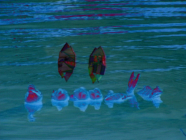 UYVY DV footage composited on GPU using "difference" op.
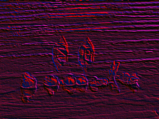 Additional processing on GPU.
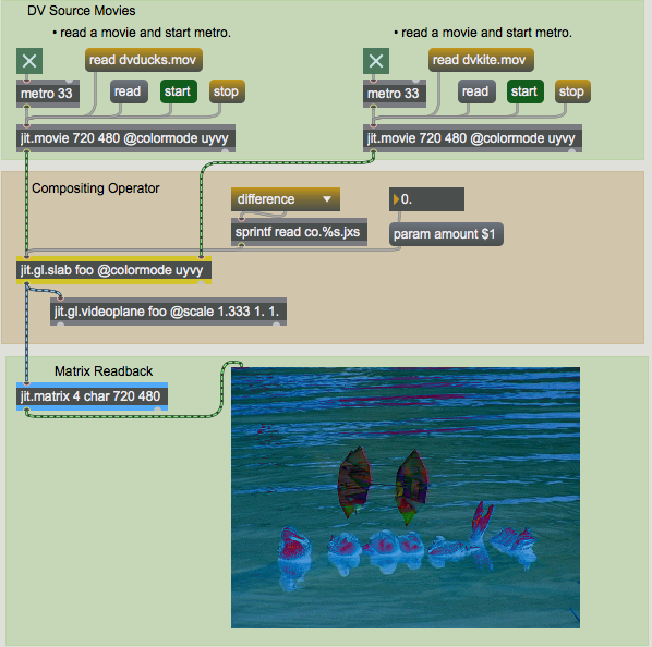 Matrix readback from GPU.