Basic Performance SetupDrawing in OpenGL using jit.gl.sketchJitter Tutorials
Tutorial 39: Spatial Mapping
In this tutorial, we will look at ways to remap the spatial layout of cells in a Jitter matrix using a second matrix as a spatial map. Along the way, we’ll investigate ways to generate complete maps through the interpolation of small datasets as well as ways to use mathematical expressions to fill a Jitter matrix with values.
Jitter matrices can be remapped spatially using lookup tables of arbitrary complexity. In Tutorial 12, we learned that the jit.charmap object maps the cell values (or color information) of one Jitter matrix based on a lookup table provided by a second Jitter matrix. In a similar fashion, the jit.repos object takes a Jitter matrix containing spatial values that it then uses as a lookup table to rearrange the spatial positions of cells in another matrix.
Open the tutorial patch.
The tutorial patch shows the matrix output of a jit.movie object being processed by a new object, called jit.repos. The right inlet of jit.repos receives matrices from the output of a jit.xfade object fed by two named matrices, each of which has been given a name (stretch and cartopol) so that they share data with jit.matrix objects elsewhere in the patch. To the right of the main processing chain are two separate areas where we construct those two matrices, which will serve as our spatial maps for this tutorial.
Click the message box that reads read colorswatch.pict to load an image into the jit.movie object. Click the toggle labeled Display to start the metro object.
Notice that at this point, we only see a solid white frame appear in the jit.pwindow object at the bottom-left of the patch. This is because we haven’t loaded a spatial map into our jit.repos object.
Open the generate_stretch subpatch.Click the first box in the preset object in the area of the patch labeled Generate “stretch” matrix. You’ll see the pictslider objects snap to various positions and a gradient progressing from magenta to green appear in the jit.pwindow at the bottom of that section.
We now see a normal looking image appear in the jit.pwindow at the bottom of our patch.
The Wide World of Repos
Open the generate_stretch subpatch.Try manipulating the pictslider objects that set values in the stretch matrix. Notice that the effect is to stretch and twist our image. By manipulating the pictslider objects one at a time, we can see that they distort different areas of the screen in a 3x3 grid. Clicking the first box in the preset object will return the image to normal.Hall of mirrors.
The pictslider objects in our patch set individual cells in a 2-plane, 3x3 Jitter matrix of type long. This matrix is then upsampled with interpolation to a 320x240 matrix named stretch. This matrix contains the instructions by which jit.repos maps the cells in our incoming matrix. The interpolation here is necessary so that we can infer an entire 320x240 map from just nine specified coordinate points.
The spatial map provided to the jit.repos object in its right inlet contains a cell-by-cell description of which input cells are mapped to which output cells. The first plane (plane 0) in this matrix defines the x coordinates for the mapping; the second plane (plane 1) represents the y coordinates. For example, if the cell in the upper-left hand corner contains the values 50 75, then the cell at coordinates 50 75 from the matrix coming into the left inlet of the jit.repos object will be placed in the upper left-hand corner of the output matrix.
The following example will give us a better sense of what jit.repos is doing with its instructions:
A simple spatial map.
In this example, we have a simple single-plane 5x5 matrix filled with ascending numbers being remapped by a spatial map. Notice the correlation between the values in the spatial map and where the corresponding cells in the output matrix get their original values from in the input matrix. For example, the cell in the lower-left of the spatial map matrix reads 4 0. The cell at coordinate {4, 0} in the incoming matrix is set to value 5. As you can see, the cell in the lower-left of the output matrix contains that value as well.
Similarly, you can see that the cells comprising the middle row of the output matrix are all set to the same value (19). This is because the corresponding cells in the spatial map are all set to the same value (3 3). Cell {3, 3} in the input matrix contains the value 19; that value is then placed into that entire row in the output matrix.
In our tutorial patch, our spatial map needs to be able to contain values in a range that represents the full size (or dim) of the matrix to be processed. To this end, the pictslider ranges are set to 320 x 240. To handle numbers of this size, we need to use a matrix of type long for our spatial map. If it was of type char, we would be constrained to values in the range of 0 to 255, limiting what cells we can choose from in our spatial map. Note that in order to correctly view these long matrices in jit.pwindow objects we use the jit.clip object to constrain the values in the matrix before viewing to the same range as char matrices.
Technical Note: The default behavior of jit.repos is to interpret the spatial map as a matrix of absolute coordinates, i.e. a literal specification of which input cells map to which output cells. The mode attribute of jit.repos, when set to 1, places the object in relative mode, wherein the spatial map contains coordinates relative to their normal position. For example, if cell {15, 10} in the spatial map contained the values -3 7, then a jit.repos object working in relative mode would set the value of cell {15, 10} in the output matrix to the contents of cell {12, 17} in the input matrix (i.e. {15-3, 10+7}).
Play around some more with the pictslider objects to get a better feel for how jit.repos is working. Notice that if you set an entire row (or column) of pictslider objects to approximately the same position you can “stretch” an area of the image to cover an entire horizontal or vertical band in the output image. If you set the pictslider objects in the left columns to values normally contained in the right columns (and vice versa), you can flip the image on its horizontal axis. By doing this only part-way, or by positioning the slider values somewhere in between where they sit on the “normal” map (as set by the preset object) you can achieve the types of spatial distortion commonplace in funhouse mirrors, where a kink in the glass bends the reflected light to produce a spatial exaggeration.
Spatial Expressions
Now that we’ve experimented with designing spatial maps by hand, as it were, we can look at some interesting ways to generate them algorithmically.
Open the generate_cartopol subpatch.Click the button labeled Generate. Set the number box labeled Crossfade (attached to the trigger object in the main part of the patch) to 1.0.Lollipop space.
The cartopol spatial map has been set by a mathematical expression operated on the output of the jit.gencoord object by the jit.expr object. The results of this expression, performed on float32 Jitter matrices, are then copied into a long matrix that serves as our spatial map. This spatial map causes jit.repos to spatially remap our incoming matrix from Cartesian to polar space, so that the leftmost edge of our incoming matrix becomes the center of the outgoing matrix, wrapping in a spiral pattern out to the final ring, which represents the rightmost edge of the input matrix. The boundmode attribute of jit.repos tells the object to wrap coordinates beyond that range back inwards, so that the final edge of our output image begins to fold in again towards the left side of the input image.
The jit.gencoord object outputs a simple Cartesian map of floating-point values; when you multiply the values in the matrix by the dim of the matrix, you can easily get coordinates which literally correspond to the locations of the cells, as shown in this illustration:
Normal Cartesian map.
The scale and offset attributes of jit.gencoord allow us to manipulate the range of values put out by the object, saving us the step of using multiple jit.op objects to get our Cartesian map into the range we want. For our equation to work, we want our starting map to be in the range of {-1, 1} across both dimensions (hence we multiply the normal Cartesian space by 2 and offset it by -1).
The jit.expr object takes the incoming matrix provided by jit.gencoord and performs a mathematical expression on it, much as the Max vexpr object works on lists of numbers. The expr attribute of the jit.expr object defines the expression to use. The in[i].p[j] notation tells jit.expr that we want to operate on the values contained in plane j of the matrix arriving at inlet i. The dim[i] keyword returns the size of the dimension i in the matrix. In our case, the notation dim[0] would resolve to 320; dim[1] would resolve to 240.
Note that there are actually two mathematical expressions defined in the message box setting the expr attribute. The first defines the expression to use for plane 0 (the x coordinates of our spatial map), the second sets the expression for plane 1 (the y coordinates).
Placed in a more legible notation, the jit.expr expression for plane 0:
hypot(in[0].p[0]*in[1]\,in[0].p[1]*in[2])*dim[0]
works out to something like this, if x is the value in plane 0 of the input, y is the value in plane 1 of the input, and a and b are the values in the number box objects attached to the second and third inlets of the jit.expr object:
Therefore, we can see that we are filling the x (plane 0) values of our spatial map with numbers corresponding to the length of the hypotenuse of our coordinates (i.e. their distance from the center of the map), while we set the y (plane 1) values to represent those values’ angle (Ø) around the origin.
In the lower-right section of the tutorial patch, change the number box objects attached to the jit.expr object. Note that they allow you to stretch and shrink the spatial map along the x and y axes.
The jit.expr object can take Max numerical values (int or float) in its inlets in lieu of matrices. Thus the in[1] and in[2] notation in the expr attribute refers to the numbers arriving at the middle and right inlets of the object.
Technical Note: The jit.expr object parses the mathematical expressions contained in the expr attribute as individual strings (one per plane). As a result, each individual expression should be contained in quotes and commas need to be escaped by backslash (\) characters. This is to prevent Max from atomizing the expression into a list separated by spaces or a sequence of messages separated by commas. We can gain some insight into how jit.expr parses its expressions by turning on the verbose attribute to the object (as we do in this tutorial). When an expr attribute is evaluated, the object prints the expression’s evaluation hierarchy to the Max Console so we can see exactly how the different parts of the expression are tokenized and interpreted.
Open the patcher object labeled steps. Click through the different expressions contained in the message boxes, each of which shows a simpler stage of how we computed the cartopol map. The norm[i] and snorm[i] notation essentially replicates the function of jit.gencoord here, generating a map of Cartesian values (0 to 1) or signed Cartesian values (-1 to 1) across the specified dimension.Different stages of the Cartesian-to-polar mapping: (a) normal map, (b) normal map scaled and offset to a signed {-1, 1} range, (c) hypotenuse only, (d) theta only
An important thing to notice with this subpatch is that the message box objects are directly connected to the jit.matrix object in the main patch. The exprfill message to jit.matrix allows us to fill a Jitter matrix with values from a mathematical expression without having to resort to using jit.expr as a separate object. The syntax for the exprfill method is slightly different from the expr attribute to jit.expr: the first argument to exprfill is the plane to fill with values, so two exprfill messages (separated by commas) are necessary to generate the spatial map) using this method.
Still Just Matrices
Slowly change the number box attached to the trigger object on the left of the patch from 1 to 0 and back again.A partial cross-fade of the two spatial maps used in this tutorial.
The number box controls the xfade attribute of the jit.xfade object directly attached to the jit.repos object at the heart of our processing chain. As a result, we can smoothly transition from our manually defined spatial map (the stretch matrix) to our algorithmically defined one (the cartopol matrix). The ability to use Jitter processing objects to composite different spatial maps adds another layer of potential flexibility. Because the two matrices containing our maps have the same typology (type, dim, and planecount) they can be easily combined to make an infinite variety of composites.
Summary
The jit.repos object processes an input matrix based on a spatial map encoded as a matrix sent to its second inlet. The default behavior is for jit.repos to process matrices spatially using absolute coordinates, such that the cell values in the second matrix correspond to coordinates in the input matrix whose cell values are copied into the corresponding position in the output matrix.
Spatial maps can be created by setting cells explicitly in a matrix and, if desired, upsampling with interpolation from a smaller initial matrix. Maps can also be created by generating matrices through algorithmic means, such as processing a “normal” Cartesian map generated by a jit.gencoord object through a mathematical expression evaluated by a jit.expr object. The jit.expr object takes strings of mathematical expressions, one per plane, and parses them using keywords to represent incoming cell values as well as other useful information, such as the size of the incoming matrix. If you want to fill a Jitter matrix with the results of a mathematical expression directly, you can use the exprfill message to a jit.matrix object to accomplish the same results without having to use a separate jit.expr object.
The jit.repos object can be used with a wide variety of spatial maps for different uses in image and data processing. The ‘jitter-examples/video/spatial’ folder of the Max ‘examples’ folder contains a number of patches that illustrate the possibilities of jit.repos.
Two-dimensional storage and viewing256 point input to output mapLimit data to the range [min,max]Evaluate expressionsEvaluates a procedural basis function graphThe Jitter Matrix!In-Patcher WindowPlay or edit a movieReposition spatiallyCrossfade between 2 matrices
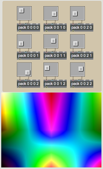 Hall of mirrors.
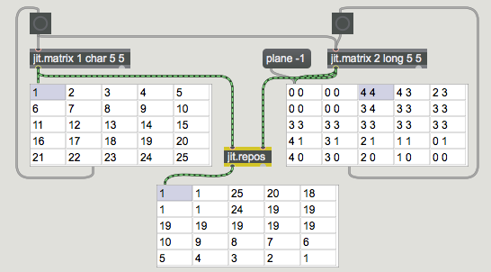 A simple spatial map.
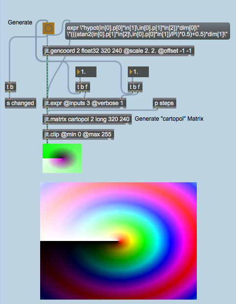 Lollipop space.
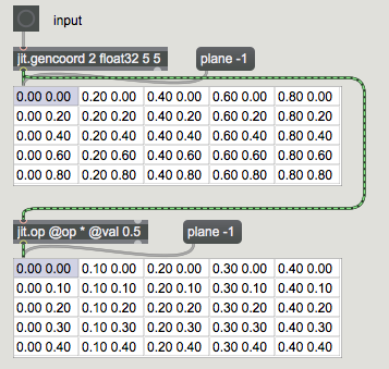 Normal Cartesian map.
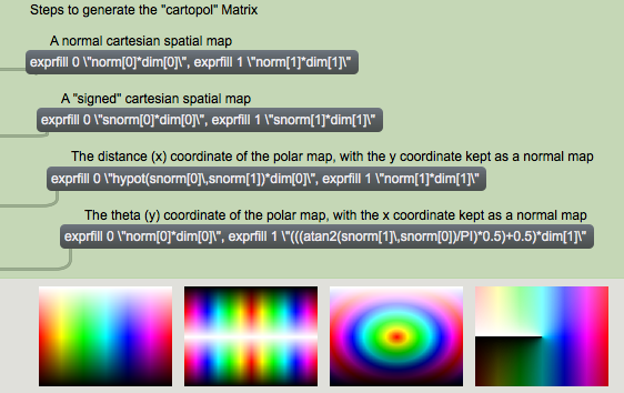 Different stages of the Cartesian-to-polar mapping: (a) normal map, (b) normal map scaled and offset to a signed {-1, 1} range, (c) hypotenuse only, (d) theta only
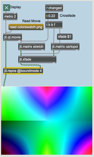 A partial cross-fade of the two spatial maps used in this tutorial.